Module 07. Using Third Party Packages
Lecture Date 1: October 4, 2021 - Monday Slides-1
Lecture Date 2: October 6, 2021 - Wednesday Slides-2
 DataCamp Chapters:
 Introduction to Python -> NumPy
Intermediate Python -> Matplotlib
In this lecture, we will delve into using third party packages in Python. After learning how to use package managers, we will install and use two packages, namely NumPy and Matplotlib, which are of great use for modeling and simulation. In the NumPy part, we will learn creating arrays and matrices with zeros, default value, or random values. Similar to lists, NumPy arrays can be sliced which will be covered. We will see useful NumPy features such as element-wise operations and very simple statistics. The final part of the NumPy is spaces and ranges, which are fundamental for many modeling tasks especially when generating timesteps and numerical ranges. For plotting purposes, we will learn basic Matplotlib concepts and example plots. You will also study the same topics on DataCamp.
Table of contents:
1. NumPy
1.1. Importing numpy
import numpy as np
1.2. Creating arrays
vec = np.zeros( 5 )
vec
array([0., 0., 0., 0., 0.])
vec = np.full(5, 1.0)
vec
array([1., 1., 1., 1., 1.])
np.array([4,4,1,6])
array([4, 4, 1, 6])
np.array([4,4,1,6.0])
array([4., 4., 1., 6.])
np.array([4,4,1,"6"])
array(['4', '4', '1', '6'], dtype='<U21')
1.3. Creating arrays w/ random values
vec = np.random.random(4)
vec
array([0.75501967, 0.0262822 , 0.07794013, 0.89892791])
vec = np.random.randint(1,6,4)
vec
array([3, 3, 4, 1])
vec = np.random.random(100)
vec
array([0.35846469, 0.77451298, 0.15087849, 0.82660523, 0.17576449,
       0.71226487, 0.17593594, 0.39902983, 0.23795018, 0.92141048,
       0.0117508 , 0.91708938, 0.54539842, 0.74121229, 0.71757155,
       0.16266148, 0.26903274, 0.76150291, 0.94069854, 0.12357852,
       0.18019493, 0.6819162 , 0.91685318, 0.79641327, 0.98860359,
       0.57408123, 0.94118066, 0.93568715, 0.7397282 , 0.64016067,
       0.91817016, 0.78376564, 0.59234063, 0.13711589, 0.65232768,
       0.18254546, 0.5227466 , 0.17327965, 0.59023643, 0.80916433,
       0.81127616, 0.44741294, 0.39846879, 0.3209138 , 0.24765607,
       0.1818303 , 0.7226836 , 0.45560892, 0.69149294, 0.59434258,
       0.98837328, 0.9480647 , 0.96933242, 0.63722027, 0.38460225,
       0.93370954, 0.02181841, 0.52460362, 0.33157321, 0.43547651,
       0.18468617, 0.01223185, 0.16440112, 0.61954091, 0.93681645,
       0.19508115, 0.97413405, 0.81792091, 0.06204738, 0.65529382,
       0.36807633, 0.17149767, 0.85520454, 0.11964864, 0.97031266,
       0.79627894, 0.11243948, 0.04428104, 0.62859646, 0.9106482 ,
       0.13326481, 0.25007363, 0.66340838, 0.77973629, 0.29062973,
       0.68698655, 0.07624197, 0.35833944, 0.05928828, 0.50483135,
       0.71256336, 0.8095939 , 0.92364977, 0.35901624, 0.92266662,
       0.12871028, 0.17891925, 0.49346012, 0.4135263 , 0.36438616])
1.4. Slicing arrays
vec[0]
0.35846469065173314
vec[:4]
array([0.35846469, 0.77451298, 0.15087849, 0.82660523])
vec[-1]
0.36438616175314675
1.5. Matrix
mat = np.zeros((2,3))
print(mat)
[[0. 0. 0.]
 [0. 0. 0.]]
mat = np.random.random((2,3))
print(mat)
[[0.477366   0.90993792 0.16192207]
 [0.09071276 0.13224813 0.98704175]]
1.6. Control printing
np.set_printoptions(precision=3)
mat
array([[0.477, 0.91 , 0.162],
       [0.091, 0.132, 0.987]])
1.7. Slicing matrices
mat[0,0]
0.4773660008379135
mat[0]
array([0.477, 0.91 , 0.162])
mat[:,0]
array([0.477, 0.091])
np.set_printoptions(precision=2)
mat2 = np.random.random((10,10))
print(mat2)
[[0.19 0.95 0.12 0.22 0.29 0.44 0.7  0.63 0.09 0.54]
 [0.65 0.29 0.37 0.54 0.88 0.31 0.88 0.21 0.07 0.31]
 [0.84 0.01 0.92 0.5  0.62 0.22 0.78 0.44 0.44 0.2 ]
 [0.27 0.86 0.36 0.66 0.19 0.57 0.44 0.96 0.31 0.12]
 [0.29 0.63 0.22 0.   0.27 0.63 0.98 0.48 0.53 0.64]
 [0.49 0.59 0.42 0.3  0.9  0.53 0.13 0.84 0.51 0.83]
 [0.01 0.21 0.34 0.76 0.27 0.48 0.11 0.73 0.64 0.33]
 [0.22 0.09 0.4  0.45 0.16 0.9  0.22 0.11 0.18 0.18]
 [0.38 0.6  0.68 0.66 0.26 0.95 0.73 0.42 0.71 0.78]
 [0.79 0.95 0.04 0.23 0.1  0.79 0.25 0.74 0.98 0.57]]
print(mat2[1:4])
[[0.65 0.29 0.37 0.54 0.88 0.31 0.88 0.21 0.07 0.31]
 [0.84 0.01 0.92 0.5  0.62 0.22 0.78 0.44 0.44 0.2 ]
 [0.27 0.86 0.36 0.66 0.19 0.57 0.44 0.96 0.31 0.12]]
mat2[2:,2:4]
array([[0.92, 0.5 ],
       [0.36, 0.66],
       [0.22, 0.  ],
       [0.42, 0.3 ],
       [0.34, 0.76],
       [0.4 , 0.45],
       [0.68, 0.66],
       [0.04, 0.23]])
v = [3,4,2]
h = [1,0,5]

mat2[v,h]
array([0.507, 0.48 , 0.453])
1.8. Setting values
mat3 = np.zeros((4,5))
print(mat3)
[[0. 0. 0. 0. 0.]
 [0. 0. 0. 0. 0.]
 [0. 0. 0. 0. 0.]
 [0. 0. 0. 0. 0.]]
mat3[1:3, 2:5] = ((1,2,3), (4,5,6))
print(mat3)
[[0. 0. 0. 0. 0.]
 [0. 0. 1. 2. 3.]
 [0. 0. 4. 5. 6.]
 [0. 0. 0. 0. 0.]]
1.9. Comparison
vec = np.random.random(4)
print(vec)
[0.14 0.61 0.02 0.63]
vec > 0.3
array([False, True, False, True])
np.where(vec > 0.3)
(array([1, 3]),)
a_matrix = np.random.random((3,4))
print(a_matrix)
[[0.85 0.86 0.53 0.49]
 [0.53 0.5  0.84 0.01]
 [0.34 0.58 0.74 0.9 ]]
np.where(a_matrix > 0.3)
(array([0, 0, 0, 0, 1, 1, 1, 2, 2, 2, 2]),
 array([0, 1, 2, 3, 0, 1, 2, 0, 1, 2, 3]))
1.10. Generating many random values
for i in range(200):
    print(np.random.randint(0,6,1), end=",")
[0],[0],[2],[4],[1],[0],[4],[0],[3],[0],[2],[5],[1],[1],[3],[1],[4],[5],[2],[3],[4],[2],[5],[1],[0],[4],[3],[5],[4],[3],[3],[5],[3],[3],[3],[5],[5],[1],[0],[1],[4],[1],[5],[2],[5],[3],[0],[5],[3],[5],[4],[2],[5],[0],[0],[3],[0],[2],[4],[0],[0],[0],[3],[4],[4],[4],[3],[5],[4],[4],[5],[2],[5],[2],[3],[1],[1],[0],[4],[5],[5],[1],[3],[5],[0],[4],[5],[4],[2],[1],[2],[1],[5],[2],[2],[3],[3],[5],[5],[4],[1],[5],[5],[5],[5],[3],[5],[5],[5],[1],[3],[3],[1],[3],[0],[4],[1],[3],[0],[0],[2],[0],[0],[0],[1],[2],[5],[5],[3],[2],[0],[1],[4],[5],[4],[3],[5],[3],[5],[0],[5],[0],[4],[4],[4],[5],[3],[5],[2],[3],[5],[3],[5],[0],[4],[3],[0],[5],[0],[0],[4],[0],[3],[1],[2],[1],[0],[5],[4],[3],[3],[3],[2],[2],[3],[3],[0],[4],[3],[2],[2],[1],[2],[2],[0],[4],[0],[3],[4],[0],[1],[3],[5],[3],[4],[4],[1],[1],[0],[2],
np.random.randint(0,6,200)
array([5, 1, 5, 1, 4, 1, 3, 4, 3, 5, 5, 2, 5, 0, 0, 2, 4, 3, 3, 4, 5, 1,
       5, 0, 0, 3, 2, 4, 3, 3, 0, 3, 5, 2, 5, 5, 3, 5, 3, 5, 2, 4, 3, 5,
       5, 2, 4, 3, 2, 5, 5, 5, 0, 2, 1, 2, 3, 1, 4, 0, 0, 3, 4, 2, 0, 4,
       0, 5, 1, 1, 0, 3, 4, 0, 3, 2, 5, 0, 0, 3, 3, 1, 4, 2, 4, 4, 0, 0,
       4, 5, 5, 4, 4, 4, 4, 3, 2, 2, 2, 4, 2, 3, 5, 3, 5, 1, 0, 2, 2, 2,
       0, 2, 5, 2, 5, 5, 2, 5, 0, 0, 2, 4, 2, 5, 4, 4, 4, 2, 1, 1, 2, 4,
       2, 5, 4, 2, 1, 0, 0, 2, 0, 5, 4, 1, 0, 3, 5, 1, 2, 4, 2, 0, 4, 0,
       2, 4, 2, 2, 4, 4, 1, 5, 4, 2, 3, 1, 1, 1, 5, 4, 3, 3, 0, 0, 1, 0,
       0, 2, 4, 5, 3, 5, 5, 3, 1, 5, 1, 3, 4, 2, 4, 0, 5, 4, 3, 5, 0, 1,
       0, 0])
np.random.randint(1,7,2)
array([2, 4])
1.11. Elementwise operations
list1 = [0, 2, 4, 6, 8, 10, 12, 14, 16, 18, 20]
list2 = [1, 3, 5, 7, 9, 11, 13, 15, 17, 19, 21]
#plus operation
result = []
for item in zip(list1,list2):
    result.append(item[0]+item[1])

result
[1, 5, 9, 13, 17, 21, 25, 29, 33, 37, 41]
#multiply
result = []
for item in zip(list1,list2):
    result.append(item[0]*item[1])
result
[0, 6, 20, 42, 72, 110, 156, 210, 272, 342, 420]
#plus operation using range
result = []
for i in range(len(list1)):
    result.append(list1[i]+list2[i])

result
[1, 5, 9, 13, 17, 21, 25, 29, 33, 37, 41]
np.array(list1) + np.array(list2)
array([ 1, 5, 9, 13, 17, 21, 25, 29, 33, 37, 41])
np.array(list1) * np.array(list2)
array([ 0, 6, 20, 42, 72, 110, 156, 210, 272, 342, 420])
1.12. Dot operation
M = np.random.random((3,4))
M
array([[0.82216265, 0.73832599, 0.61855577, 0.5972113 ],
       [0.78961636, 0.88366377, 0.41433647, 0.80100396],
       [0.25190206, 0.22419015, 0.82549157, 0.19648718]])
b = np.random.random(4)
b
array([0.01368557, 0.91652063, 0.53488074, 0.94372528])
v = M.dot(b)
v
array([1.58239975, 1.79825071, 0.83589179])
1.13. Transpose and Inverse Matrix
M.T
array([[0.82216265, 0.78961636, 0.25190206],
       [0.73832599, 0.88366377, 0.22419015],
       [0.61855577, 0.41433647, 0.82549157],
       [0.5972113 , 0.80100396, 0.19648718]])
M2 = np.random.random((3,3))
M2
array([[0.82569897, 0.95879765, 0.63989802],
       [0.97742289, 0.48473993, 0.61672715],
       [0.78989802, 0.59149062, 0.58261736]])
M2_inv = np.linalg.inv(M2)
M2_inv
array([[  3.74425336,   8.18751661, -12.77923487],
       [  3.74159729,   1.10857075,  -5.28292939],
       [ -8.8749467 , -12.22588416,  24.40554721]])
M2.dot(M2_inv)
array([[ 1.00000000e+00, -9.26482757e-16, -2.19694825e-15],
       [-2.99981245e-16,  1.00000000e+00,  2.16693348e-16],
       [-5.94315269e-16, -4.96401759e-16,  1.00000000e+00]])
1.14. Summary Statistics
mat5 = np.random.random((3,10))
print(mat5)
[[0.02 0.92 0.56 0.11 0.74 0.58 0.37 0.82 0.15 0.87]
 [0.13 0.32 0.83 0.38 0.5  0.01 0.58 0.11 0.87 0.68]
 [0.63 0.28 0.71 0.99 0.17 0.05 0.39 0.63 0.42 0.04]]
mat5.sum()
13.884423482782147
mat5.mean()
0.4628141160927382
mat5.std()
0.29963058603329346
mat5.min()
0.012156748792890304
mat5.max()
0.9859403329385706
mat5.argmin()
15
mat5.argmax()
23
mat5.sum(0)
array([0.79, 1.53, 2.1 , 1.48, 1.4 , 0.64, 1.35, 1.56, 1.45, 1.59])
mat5.sum(1)
array([5.14, 4.42, 4.32])
mat5.min(0)
array([0.02, 0.28, 0.56, 0.11, 0.17, 0.01, 0.37, 0.11, 0.15, 0.04])
mat5.min(1)
array([0.02, 0.01, 0.04])
m = np.random.random((2,3))
print(m)
[[0.79 0.74 0.41]
 [0.36 0.96 0.23]]
np.sqrt(m)
array([[0.89, 0.86, 0.64],
       [0.6 , 0.98, 0.48]])
np.sin(m)
array([[0.71, 0.68, 0.4 ],
       [0.35, 0.82, 0.23]])
np.power(m,3)
array([[0.5 , 0.41, 0.07],
       [0.05, 0.89, 0.01]])
vec = np.random.random(10) * 10
vec
array([4.57032698, 0.69638588, 0.51183216, 8.73871741, 0.44382573,
       6.33950473, 5.55468013, 7.04835898, 8.74370488, 8.60587409])
vec.sum()
51.25321097696233
vec.mean()
5.125321097696233
vec.std()
3.267176360857343
vec.min()
0.4438257269716095
vec.max()
8.743704880697376
vec.argmin()
4
vec.argmax()
8
1.15. Spaces/Ranges
np.linspace(0, 2, 21)
array([0. , 0.1, 0.2, 0.3, 0.4, 0.5, 0.6, 0.7, 0.8, 0.9, 1. , 1.1, 1.2,
       1.3, 1.4, 1.5, 1.6, 1.7, 1.8, 1.9, 2. ])
np.arange(0, 2.1, 0.1)
array([0. , 0.1, 0.2, 0.3, 0.4, 0.5, 0.6, 0.7, 0.8, 0.9, 1. , 1.1, 1.2,
       1.3, 1.4, 1.5, 1.6, 1.7, 1.8, 1.9, 2. ])
2. Matplotlib
2.1. Import Matplotlib
import matplotlib.pyplot as plt
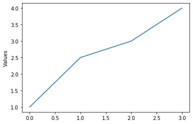
2.2. Line plot
plt.plot([1, 2.5, 3, 4])
plt.ylabel('Values')
plt.show()
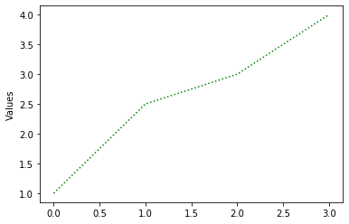
plt.plot([1,2.5,3,4],linestyle='dotted',color='green')
plt.ylabel('Values')
plt.show()
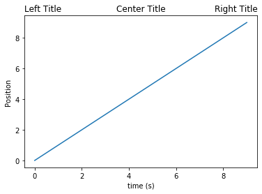
plt.plot(range(10))
plt.title('Center Title')
plt.title('Left Title', loc='left')
plt.title('Right Title', loc='right')
plt.xlabel('time (s)')
plt.ylabel('Position')
plt.show()
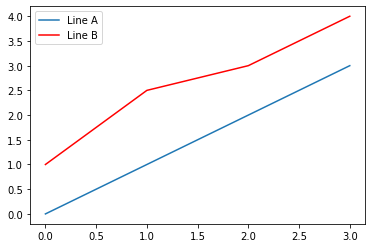
2.3. Multi line plot
plt.plot(range(4), label="Line A")
plt.plot([1,2.5,3,4], color="red", label="Line B")
plt.legend()
plt.show()
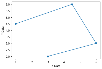
2.4. x,y line plot
x  = [1,4.5,6,3]
y  = [4.5,6,3,2]
plt.plot(x,y, marker='o')
plt.xlabel('X Data')
plt.ylabel('Y Data')
plt.show()
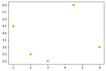
2.5. Scatter plot
x  = [1,4.5,6,3, 2]
y  = [4.5,6,3,2, 2.5]
plt.scatter(x,y,50,"y")
plt.show()
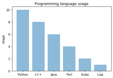
2.6. Bar plot
objects = ('Python', 'C++', 'Java', 'Perl', 'Scala', 'Lisp')
x_pos = np.arange(len(objects))
performance = [10,8,6,4,2,1]

plt.bar(x_pos, performance, align='center', alpha=0.5)
plt.xticks(x_pos, objects)
plt.ylabel('Usage')
plt.title('Programming language usage')

plt.show()
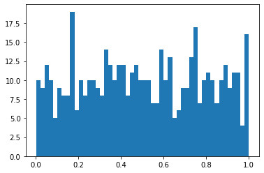
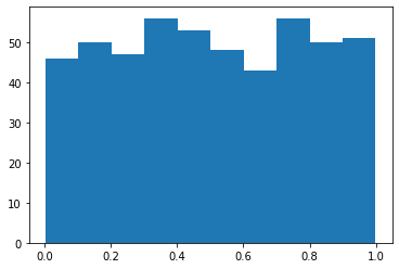
2.7. Histogram plot
vals = np.random.random(500)
plt.hist(vals)
plt.show()
plt.hist(vals,bins=50)
plt.show()