Module 08. Dynamical Systems
Lecture Date 1: October 20, 2021 - Wednesday
Lecture Date 2: October 25, 2021 - Monday
Lecture Date 3: October 27, 2021 - Wednesday
In the first two lectures of the second half, we will learn about dynamical systems and solve example questions in Python.
1. Dynamical Systems
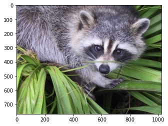
1.1. Importing packages
from scipy import misc
import matplotlib.pyplot as plt
face = misc.face()
plt.imshow(face)
plt.show()
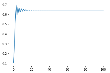
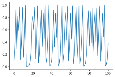
1.2. Chaotic difference equation example
import matplotlib.pyplot as plt
def chaos(r,xn):
    return r * xn * (1-xn)
# variables
r=2
x0=0.1
n = 100
r=2
x0=0.1
final_list = [x0]
for i in range(n):
    x0 = chaos(r,x0)
    final_list.append(x0)
plt.plot(final_list)
[<matplotlib.lines.Line2D at 0x7f94e9067d30>]
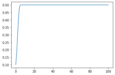
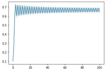
r=2.5
r=2.5
x0=0.1
final_list = [x0]
for i in range(n):
    x0 = chaos(r,x0)
    final_list.append(x0)
plt.plot(final_list)
[<matplotlib.lines.Line2D at 0x7f94c0199220>]
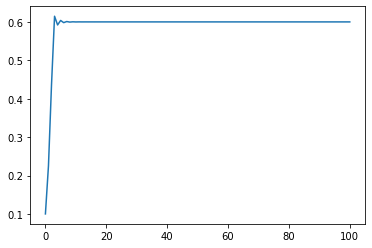
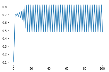
r=2.8
x0=0.1
r=2.8
final_list = [x0]
for i in range(n):
    x0 = chaos(r,x0)
    final_list.append(x0)
plt.plot(final_list)
[<matplotlib.lines.Line2D at 0x7f94f8339c10>]
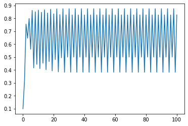
r=3.
x0=0.1
r=3.
final_list = [x0]
for i in range(100):
    x0 = chaos(r,x0)
    final_list.append(x0)

plt.plot(final_list)
[<matplotlib.lines.Line2D at 0x7f94f8352970>]
r=3.3
x0=0.1
r=3.3
final_list = [x0]
for i in range(100):
    x0 = chaos(r,x0)
    final_list.append(x0)

plt.plot(final_list)
[<matplotlib.lines.Line2D at 0x7f94d87336d0>]
r=3.5
x0=0.1
r=3.5
final_list = [x0]
for i in range(100):
    x0 = chaos(r,x0)
    final_list.append(x0)

plt.plot(final_list)
[<matplotlib.lines.Line2D at 0x7f94a81619a0>]
r=4.0
x0=0.1
r=4.0
final_list = [x0]
for i in range(100):
    x0 = chaos(r,x0)
    final_list.append(x0)

plt.plot(final_list)
[<matplotlib.lines.Line2D at 0x7f94e95132e0>]
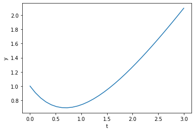
1.3. ODE Example
def dy_dt(y,t):
    return t - y
import scipy.integrate as sci
import numpy as np
y0 = 1.0
t = np.linspace(0,3,30)
y = sci.odeint(dy_dt, y0, t)
plt.plot(t,y.flatten())
plt.xlabel("t")
plt.ylabel("y")
plt.show()
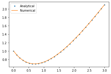
y_exact = t - 1 + 2 * np.exp(-t)
y_exact
array([1.        , 0.9068936 , 0.83310407, 0.776733  , 0.73606855,
       0.70956712, 0.69583679, 0.69362247, 0.70179239, 0.71932601,
       0.74530309, 0.77889384, 0.81935   , 0.86599685, 0.918226  ,
       0.97548883, 1.03729064, 1.10318535, 1.17277073, 1.24568406,
       1.32159829, 1.40021849, 1.48127873, 1.5645392 , 1.64978368,
       1.73681717, 1.82546387, 1.91556523, 2.00697829, 2.09957414])
plt.plot(t, y_exact,".", label="Analytical")
plt.plot(t, y,label="Numerical")
plt.legend()
plt.show()
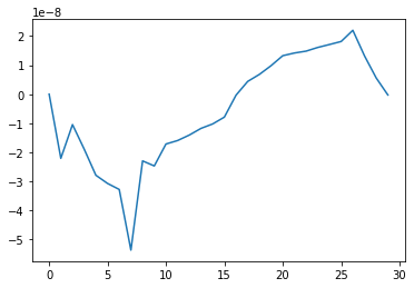
diff = y_exact - y.flatten()
len(diff)
30
diff
array([ 0.00000000e+00, -2.20936942e-08, -1.04747599e-08, -1.89222228e-08,
       -2.79155825e-08, -3.07385867e-08, -3.28044586e-08, -5.36908111e-08,
       -2.29745252e-08, -2.47152306e-08, -1.71658219e-08, -1.59589546e-08,
       -1.40732747e-08, -1.17833546e-08, -1.02491686e-08, -7.89757781e-09,
       -3.39251960e-10,  4.39486425e-09,  6.81157486e-09,  9.81517134e-09,
        1.32513973e-08,  1.41764489e-08,  1.48237629e-08,  1.60960052e-08,
        1.71045875e-08,  1.81424631e-08,  2.19980316e-08,  1.31834950e-08,
        5.59343372e-09, -2.70218958e-10])
plt.plot(diff)
plt.show()
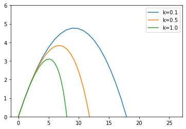
1.4. Projectile motion with air resistance
# define variables and initial values
m = 1.0
k = 0.1
g = 9.81

# the first two values are the position
# the last two values are the speed (horizontal,vertical)
v0 = np.array([0.0, 0.0, 10.0, 10.0])
def f(v, t0, k):
    # v = [u,u']
    u = v[:2]
    udot = v[2:]

    # second derivative of u
    udotdot = -k/m * udot
    udotdot[1] = udotdot[1] - g

    # v = [u',u'']
    v = np.concatenate([udot,udotdot])
    return v
k=0.1
t = np.linspace(0,3,30)
v = sci.odeint(f,v0,t,args=(k,))
k=0.5
v_k05 = sci.odeint(f,v0,t,args=(k,))
k=1.0
v_k10 = sci.odeint(f,v0,t,args=(k,))
v
array([[  0.        ,   0.        ,  10.        ,  10.        ],
       [  1.02915039,   0.97683986,   9.89708496,   8.88748843],
       [  2.04770927,   1.83918553,   9.79522907,   7.78642627],
       [  3.05578566,   2.58821535,   9.69442143,   6.69669571],
       [  4.05348741,   3.2250955 ,   9.59465126,   5.6181801 ],
       [  5.04092132,   3.75098021,   9.49590787,   4.55076405],
       [  6.01819306,   4.16701177,   9.39818069,   3.49433331],
       [  6.98540719,   4.47432068,   9.30145928,   2.44877483],
       [  7.94266723,   4.67402586,   9.20573328,   1.41397672],
       [  8.89007562,   4.76723474,   9.11099244,   0.38982825],
       [  9.82773377,   4.75504338,   9.01722662,  -0.6237802 ],
       [ 10.75574199,   4.63853646,   8.9244258 ,  -1.62695709],
       [ 11.67419962,   4.41878756,   8.83258004,  -2.61980979],
       [ 12.58320494,   4.09685918,   8.74167951,  -3.60244454],
       [ 13.48285522,   3.67380291,   8.65171448,  -4.5749665 ],
       [ 14.37324676,   3.15065951,   8.56267532,  -5.53747974],
       [ 15.25447482,   2.52845902,   8.47455252,  -6.49008728],
       [ 16.12663372,   1.80822088,   8.38733663,  -7.43289105],
       [ 16.9898168 ,   0.99095407,   8.30101832,  -8.36599196],
       [ 17.84411642,   0.07765713,   8.21558836,  -9.28948985],
       [ 18.68962402,  -0.93068163,   8.1310376 , -10.20348356],
       [ 19.52643007,  -2.03308409,   8.04735699, -11.1080709 ],
       [ 20.35462412,  -3.22858219,   7.96453759, -12.00334868],
       [ 21.17429482,  -4.51621783,   7.88257052, -12.8894127 ],
       [ 21.98552987,  -5.89504278,   7.80144701, -13.76635779],
       [ 22.78841609,  -7.36411857,   7.72115839, -14.6342778 ],
       [ 23.58303941,  -8.92251638,   7.64169606, -15.4932656 ],
       [ 24.36948486, -10.56931695,   7.56305151, -16.34341313],
       [ 25.1478366 , -12.3036105 ,   7.48521634, -17.18481136],
       [ 25.91817793, -14.12449657,   7.40818221, -18.01755034]])
plt.plot(v[:,0],v[:,1],label="k=0.1")
plt.plot(v_k05[:,0],v_k05[:,1],label="k=0.5")
plt.plot(v_k10[:,0],v_k10[:,1],label="k=1.0")
plt.ylim([0,6])
plt.legend()
plt.show()